What is the BRAS

In short: I designed a score function for Backgammon that, in a single pass and without dice rolls or search, maps positions into the [0,100] range, is antisymmetric, interpretable, and works at millisecond speed. Below I share its formula, rationale, validation, and how it performs for doubling (cube) decisions.

Symbols and Notation Glossary

• Y_i, O_i (i=1..24): Number of my and opponent's checkers at point i.
• b_Y, b_O: Checkers on the bar (me/opponent).
• y_Y, y_O: Borne-off checkers (me/opponent).
• f_i: Normalized features, f_i ∈ [-1,1].
• w_i: Feature weights.
• D: Raw score (linear + interactions).
• g(D): D→S transform; tanh(D/σ).
• S_me, S_op: Final scores (0–100), S_me + S_op = 100.

TL;DR

• Closed-form: D = Σ w_i · f_i, g(D)=tanh(D/σ), σ=3.0
• Outputs: S_me = 50 + 50·g(D), S_op = 100 − S_me → guaranteed antisymmetry
• Feature set (11 total): pip, bar, off, hb, prime, anch, blot, stack, out, x1, x2 (all interpretable and normalized to [-1,1])
• Validation: Antisymmetry error ~1e−14, boundary and monotonicity tests pass, documentation examples match exactly
• Speed: ~0.78 ms/position (10k random positions)
• Doubling: g(D) is a single function → smooth, symmetric, threshold-sensitive decision zones

What Problem Are We Solving?

In Backgammon, position evaluation is usually done via search (minimax) or simulation (Monte Carlo). These are accurate but expensive: high latency, high energy consumption, weak for mobile/edge use. My goal was to produce an evaluation function that completes in a single pass, is mathematically robust (antisymmetric, bounded, monotonic), interpretable, and fast.

The Core Formula

Raw score and transformation (core definition):

D = Σ w_i · f_i
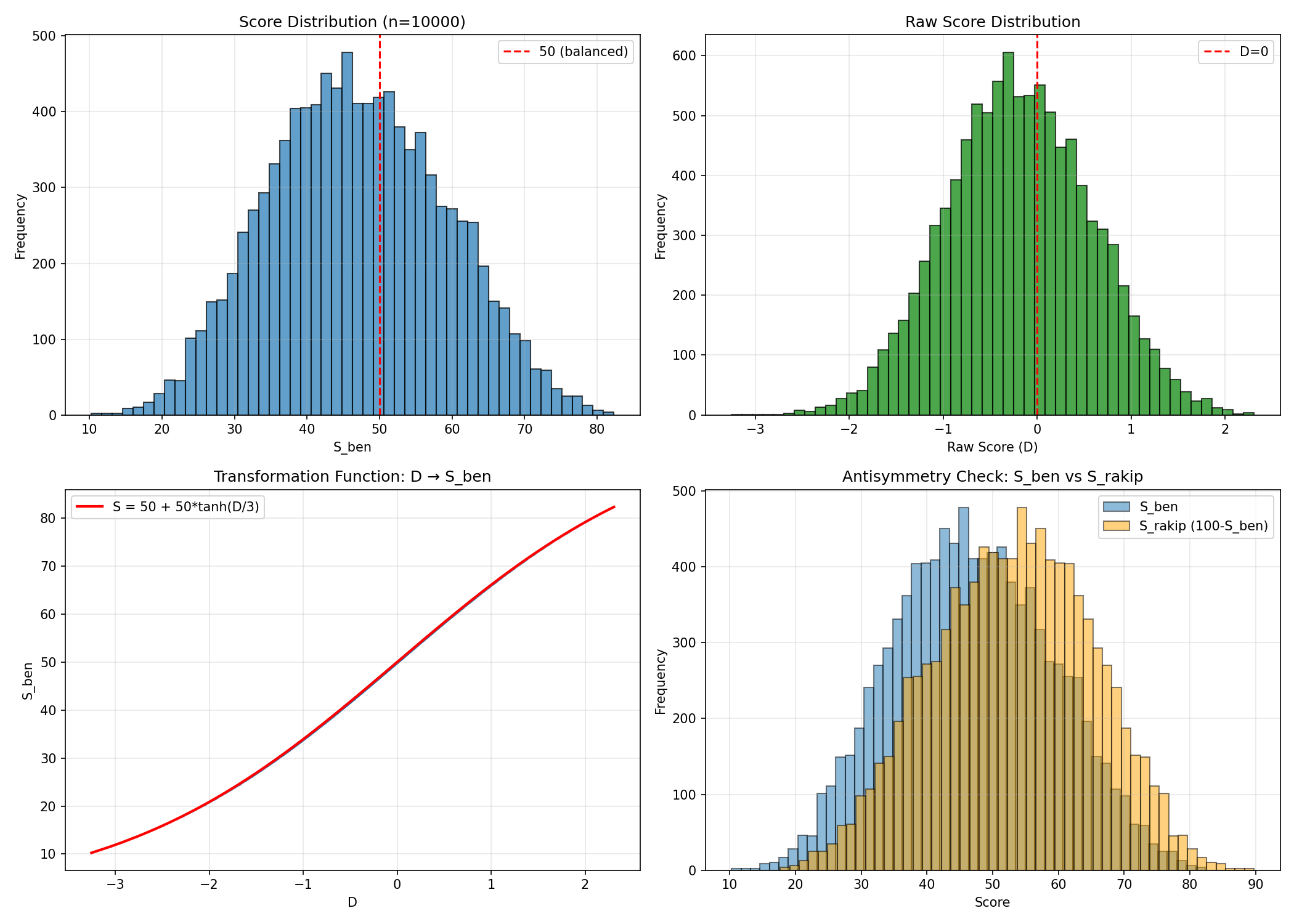
g(D) = tanh(D / σ),  σ = 3.0
S_me   = 50 + 50 · g(D)
S_op = 100 − S_me

Antisymmetry guarantee: When you flip the colors and board, all f_i signs change → D → −D → S_me ↔ 100−S_me. Therefore, S_me + S_op = 100 always holds.

Mathematical Details (In Depth)

1. Normalization and ranges (why these denominators?)

• f_pip = (PIP_O − PIP_Y) / 375

  • PIP_Y = Σ i·Y_i + 25·b_Y, PIP_O = Σ (25−i)·O_i + 25·b_O
  • For each side, PIP ∈ [0, 375] (all 15 checkers on the bar → 25×15=375; empty board → 0)
  • So difference ∈ [−375, +375]; with denominator 375, f_pip ∈ [−1,1] is guaranteed.

• f_hb = (H_Y − H_O)/6, H_· ∈ {0..6} → difference ∈ [−6,6] → [-1,1]

• f_prime = (L_Y − L_O)/6, L_· ∈ {0..6} → [-1,1]

• f_anch = (A_Y − A_O)/6, A_· ∈ {0..6} → [-1,1]

• f_blot = (W_O − W_Y)/22.5

  • W_· = Σ ρ(i)·1[·_i = 1], ρ(i) = 1.5 (1..6), 1.0 (7..18), 1.2 (19..24)
  • Worst case: one side distributes all 15 blots in my home (1..6): W_max = 15×1.5 = 22.5
  • Difference ∈ [−22.5, +22.5] → [-1,1]

• f_stack = (S_O − S_Y)/10, S_· = Σ max(·_i−5, 0)

  • Worst: 15 checkers stacked → max(15−5, 0) = 10
  • Difference ∈ [−10, +10] → [-1,1]

• f_bar = (b_O − b_Y)/15, b_· ∈ {0..15} → [-1,1]

• f_off = (y_Y − y_O)/15, y_· ∈ {0..15} → [-1,1]

• f_out = (T_Y − T_O)/12, T_· ∈ {0..12} (points 7–18, 12 in total) → [-1,1]

• f_x1 = (H_Y/6)(b_O/15) − (H_O/6)(b_Y/15)

  • Each term ∈ [0,1]; difference ∈ [−1,1]

• f_x2 = (L_Y·A_O − L_O·A_Y)/36

  • L_·, A_· ∈ {0..6} → denominator 36 assures [-1,1]

2. Antisymmetry (operator and feature-level proof):

• Flip: Ŷ_i := O_{25−i}, Ô_i := Y_{25−i}, b_Y↔b_O, y_Y↔y_O (see: bras_evaluator.py:306)
• For all features, f_i(Ŷ,Ô) = −f_i(Y,O):
  • pip: Indices and bar switch signs
  • hb/anch/out/prime/stack: Counts swap sign when side changes
  • blot: ρ*(i)=ρ(25−i) — local risk weights flip
  • bar/off: Differences change sign
  • x1/x2: Cross terms also swap sign
• Thus D(Ŷ,Ô) = −D(Y,O), S_me(Ŷ,Ô) = 100 − S_me(Y,O)

3. Transformation and derivative (sensitivity):

• g(x) = tanh(x/σ) → single function; |g|≤1
• Derivative: g'(x) = (1/σ)·sech²(x/σ); g'(0) = 1/σ ≈ 0.333 (σ=3)
• Effect on score: ∂S_me/∂D = 50·g'(D)
  • Near D=0: ∂S_me/∂D ≈ 16.67 (high sensitivity; saturates near extremes)
• Saturation intuition: |D|≈3 → |g|≈tanh(1)≈0.761 → S≈50±38

4. Monotonicity: sample derivatives

• Increase pip difference R=PIP_O−PIP_Y:

  • ∂S_me/∂R = 50·g'(D)·w_pip/375 > 0 (see: docs/ras_mathematical_foundations.md)

• Increase my bar b_Y:

  • ∂S_me/∂b_Y = −50·g'(D)·(w_bar/15 + (w_x1·H_O)/(6·15)) < 0 (negative)

5. Interpretation of weights (scale):

• Each w_i is “change in D per unit of feature”; score sensitivity is ~50·g'(D)·w_i
• Eg. D≈0, w_pip=2.2 → 50·(1/3)·2.2/375 ≈ 0.097 score/PIP unit difference

> Visualization suggestion: plot D→S curve and g’(D) (sensitivity) together to show high central sensitivity and extreme saturation.

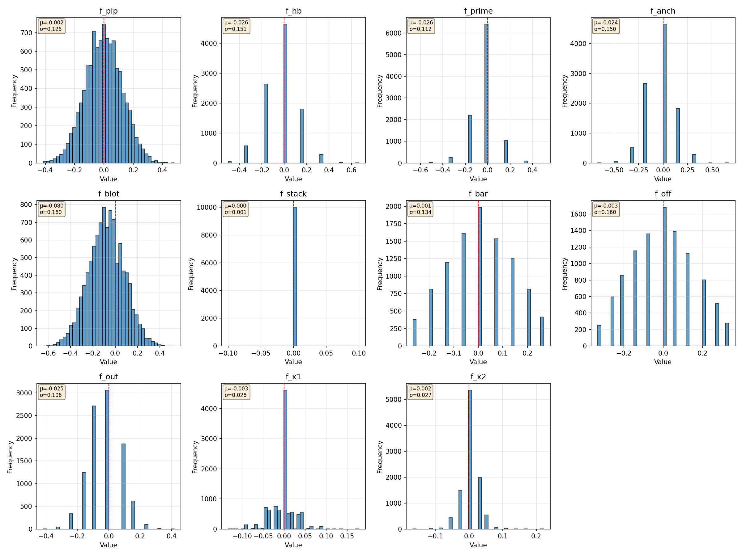
Features (f_i)

• pip: pip difference (across all phases)
• bar: bar disadvantage (very strong signal)
• off: bear-off progress (endgame speed)
• hb: home board strength (hitting/jailing)
• prime: longest prime (movement restriction)
• anch: number of anchors in opponent's home (back game security)
• blot: regionally weighted blot risk
• stack: penalty for >5 checkers stacked (flexibility loss)
• out: midboard (7–18) control
• x1: hb × bar synergy
• x2: prime × anchor interaction (dampened via negative weight)

Weights and definitions as in the implementation: bras_evaluator.py:55, detailed maths: docs/ras_mathematical_foundationd.md.

Sample 2 from docs, summary:

• f_pip ≈ +0.0427, f_blot ≈ −0.0311, f_bar ≈ −0.0667, f_out ≈ −0.0833, f_x1 ≈ −0.0111
• With weights: D ≈ −0.1265 → S_me ≈ 47.893, S_op ≈ 52.107
• Code matches: bras_evaluator.py example and test_bras.py:192

S→p(win) Calibration

The S scale (0–100) is ideal for human-readability but is not a direct “win probability.” With real-game or simulation labels (win=1/lose=0), you can calibrate S → p(win) via a simple mapping.

Recommendation: Isotonic regression (monotonic calibration)

Steps (summary):

• Collect labeled data: pairs (S_me, outcome) (outcome ∈ {0,1})
• Map S_me values [0,100] → [0,1] (e.g., S' = S_me/100)
• Learn p̂ = h(S') using isotonic regression
• Plot reliability curve, report Brier and log-loss

Sample code (adapt to your data):

import numpy as np, pandas as pd
from sklearn.isotonic import IsotonicRegression
import matplotlib.pyplot as plt

# df: results from games; S_me (0..100), outcome ∈ {0,1}
df = pd.read_csv('my_games.csv')
S = df['S_me'].values / 100.0
y = df['outcome'].values

iso = IsotonicRegression(out_of_bounds='clip')
p_hat = iso.fit_transform(S, y)

# Reliability curve
bins = np.linspace(0, 1, 11)
bucket = np.digitize(S, bins) - 1
cal = pd.DataFrame({'S': S, 'y': y, 'p': p_hat, 'b': bucket})
grp = cal.groupby('b').agg(S_mean=('S','mean'), y_mean=('y','mean'), p_mean=('p','mean'))

plt.plot(grp['S_mean'], grp['y_mean'], 'o-', label='Empirical')
plt.plot(grp['S_mean'], grp['p_mean'], 'x--', label='Calibrated')
plt.plot([0,1],[0,1],'k:', label='Perfect')
plt.xlabel('S/100'); plt.ylabel('p(win)'); plt.legend(); plt.grid(alpha=.3)
plt.tight_layout(); plt.savefig('ds_analysis/14_calibration_curve.png', dpi=150)

Notes:

• S is not equal to p(win) by default; calibration aligns it to real data.
• When σ or w gets updated, recalibrate for best accuracy.

Cube (Doubling) Threshold Guide (Money Game)

Doubling decisions are by nature thresholded. Using this function’s smooth mapping from D to S, here’s a practical guide for money game:

• Early “double consideration”: D ≳ 0.5 → S_me ≈ 50 + 50·tanh(0.5/3) ≈ 54–55
• Live cube window: D ≈ 1.0–1.5 → S_me ≈ 65–70 (position & volatility dependent)
• Drop zone: D ≳ 2.0–2.5 → S_me ≈ 80+ (opponent passing starts to make sense)

Notes:

• Thresholds depend on game phase and hit/contact dynamics; hb/prime/anch combos affect volatility.
• By antisymmetry, opponent thresholds are symmetric: read as S_op = 100 − S_me.
• You should recalibrate these with your own data, e.g., ds_analysis_doubling2/dataset.csv.

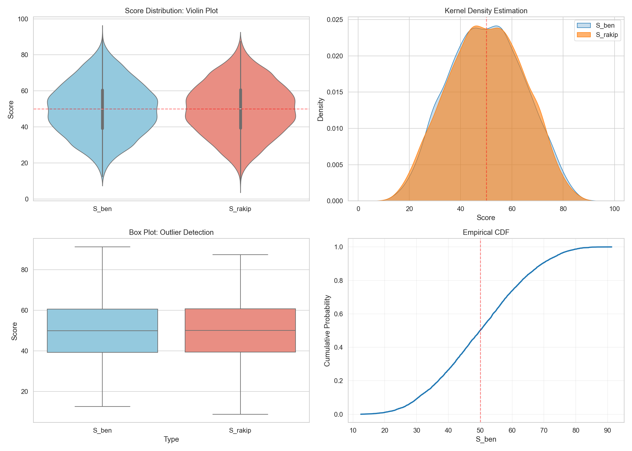
Optional visuals:

• ds_analysis_doubling2/01_score_distributions.png: Distribution context
• ds_analysis_doubling2/07_statistical_tests.png: Statistical consistency
• ds_analysis_doubling2/08_feature_importance.png: Feature effects

Integration: Engine and Decision Flow

This section covers the minimal building blocks and sample code for engine integration.

Move Ordering (Fast Sorting)

Idea: Score all child positions from legal moves using compute_score, then search best-first.

from tavla_evaluator import TavlaEvaluator

def order_moves(current_position, legal_moves, apply_move_fn, top_k=None):
    e = TavlaEvaluator()
    scored = []
    for m in legal_moves:
        child = apply_move_fn(current_position, m)  # update position
        S_me, _ = e.compute_score(child)
        scored.append((m, S_me))
    scored.sort(key=lambda t: t[1], reverse=True)
    return scored if top_k is None else scored[:top_k]

Note: In expensive search/simulation, this order accelerates pruning (best branches expand first).

Doubling Decision Flow (Simple Flow)

[Position] → compute D, S_me
    |-- S_me ≥ S_drop → Double → Opponent: Pass (profit ↑)
    |-- S_live_low ≤ S_me < S_drop → Double suggested (check position/volatility)
    |-- S_me < S_live_low → No double (play on)

Suggested initial thresholds (money game):

• S_live_low ≈ 62–65, S_drop ≈ 80

Warning: Thresholds depend on game/target; recalibrate with your data. For match play, score/equity needs adjustment.

Implementation (Python)

• Feature extraction: bras_evaluator.py:47
• Raw score: compute_raw_score → bras_evaluator.py:254
• Transformation: g_transform → bras_evaluator.py:257 (σ=3)
• Full score: compute_score → bras_evaluator.py:267
• Color/board flip (invariance test): flip_position → bras_evaluator.py:306

Sample positions (match docs): bras_evaluator.py:327, bras_evaluator.py:349

Why This Design?

• Antisymmetric and neutral: Works for both colors, interpretation preserved under flip.
• Closed form and fast: No search/simulation; single path evaluation.
• Interpretable: Each feature ties clearly to game intuition.
• Stable: tanh saturates at extremes, smooth/monotonic in center.

Tests: “I Built It, I Broke It; I Trust If It Passes”

All tests in test_bras.py; auto-generator covers boundaries, monotonicity, and edge cases.

• Antisymmetry (N=1000): S_me + S_op = 100, after flip S_me' = S_op; max error ~1e−14 (test_bras.py:139)
• Documentation examples: Opening S=50.000; contact example D≈−0.1265, S≈47.893 (tolerance < 1e−2) (test_bras.py:192)
• Feature bounds: Each f_i ∈ [-1,1] (no violations) (test_bras.py:240)
• Score bounds: S ∈ [0,100] (no violations) (test_bras.py:274)
• Monotonicity: Pip↑ ⇒ S_me↑; My bar↑ ⇒ S_me↓ (test_bras.py:303)
• Edge cases: All bar, all off, max stack; antisymmetry held (test_bras.py:402)

Output and performance:

• 10,000 random positions: total ~7.8s → ~0.78 ms/position
• For comparison: MCTS (1000 sims) ~100–500 ms/move → 100–600× faster

Statistical Analysis & Visuals

Produced EDA, correlations, importance (|w|·std), transformation behavior and sensitivity analyses.

Highlights:

• Score & transformation: IMG/bras_analysis_scores.png
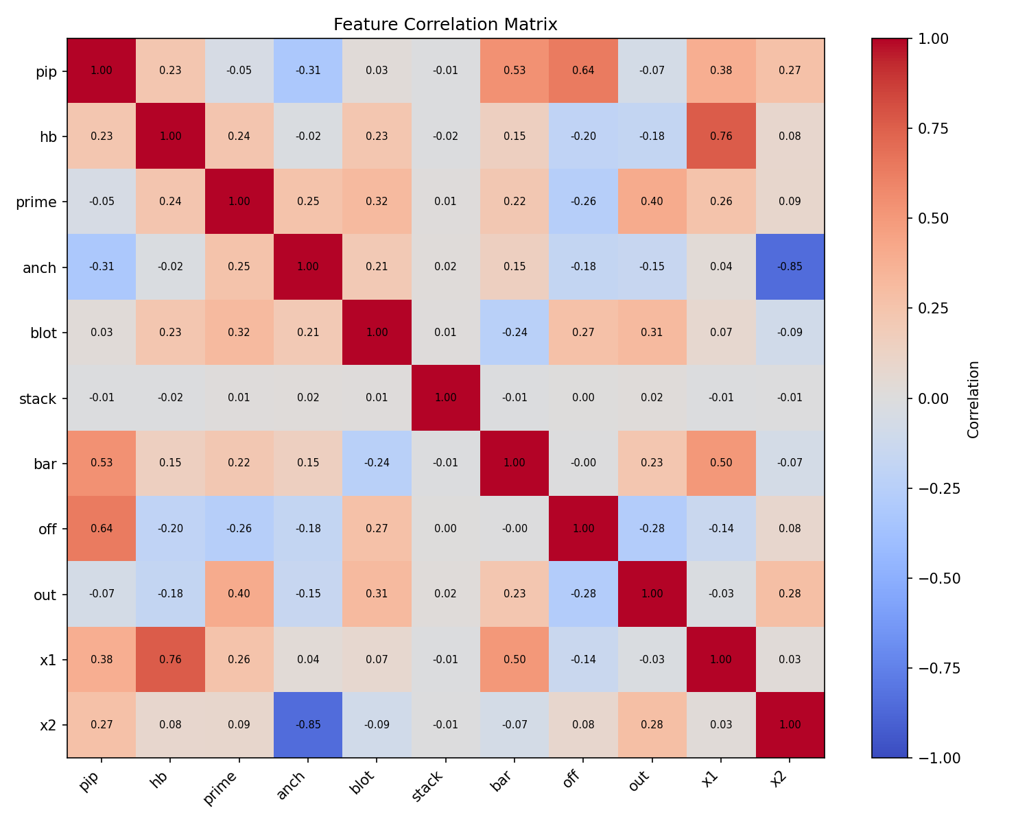
• Feature histograms: IMG/bras_analysis_features.png
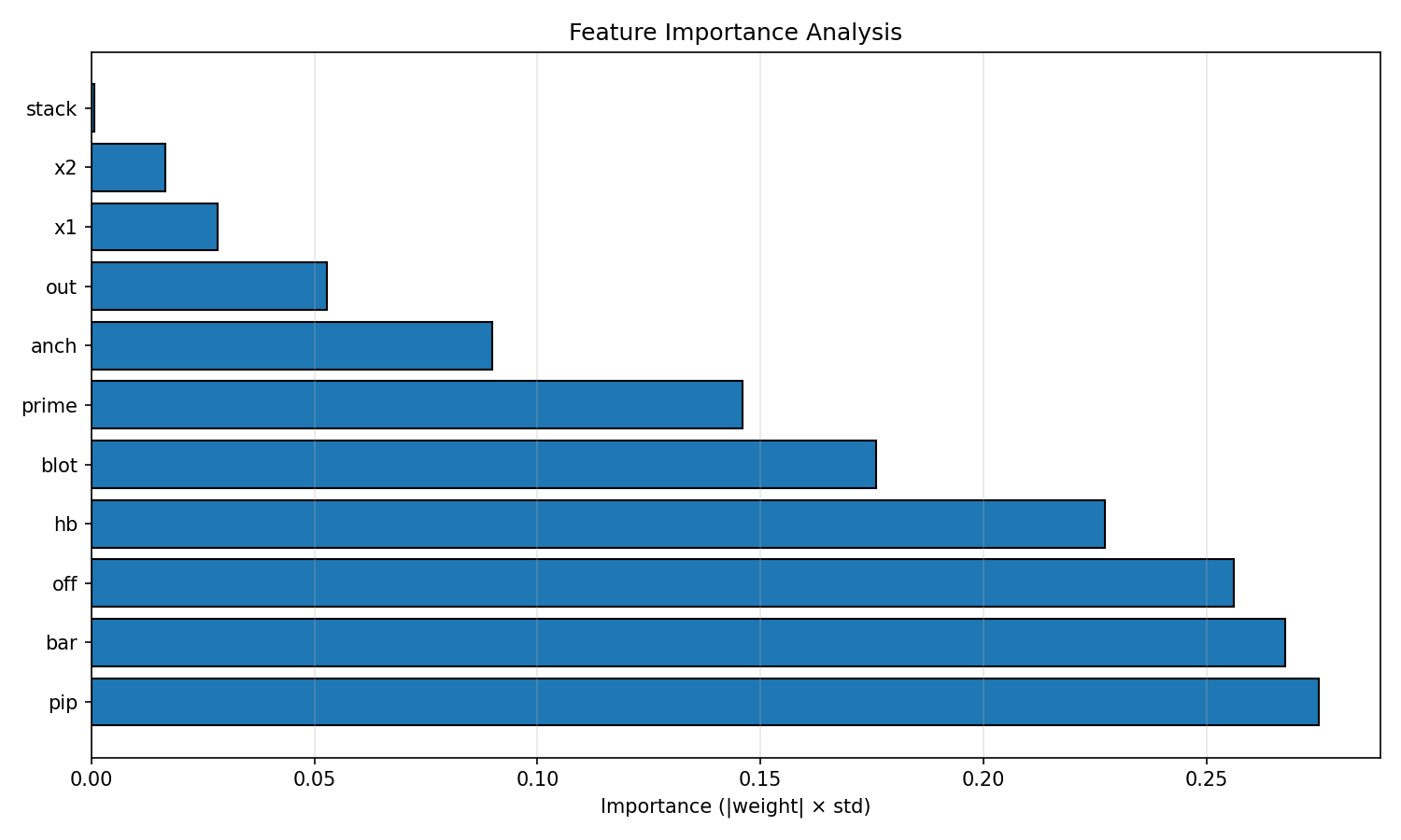
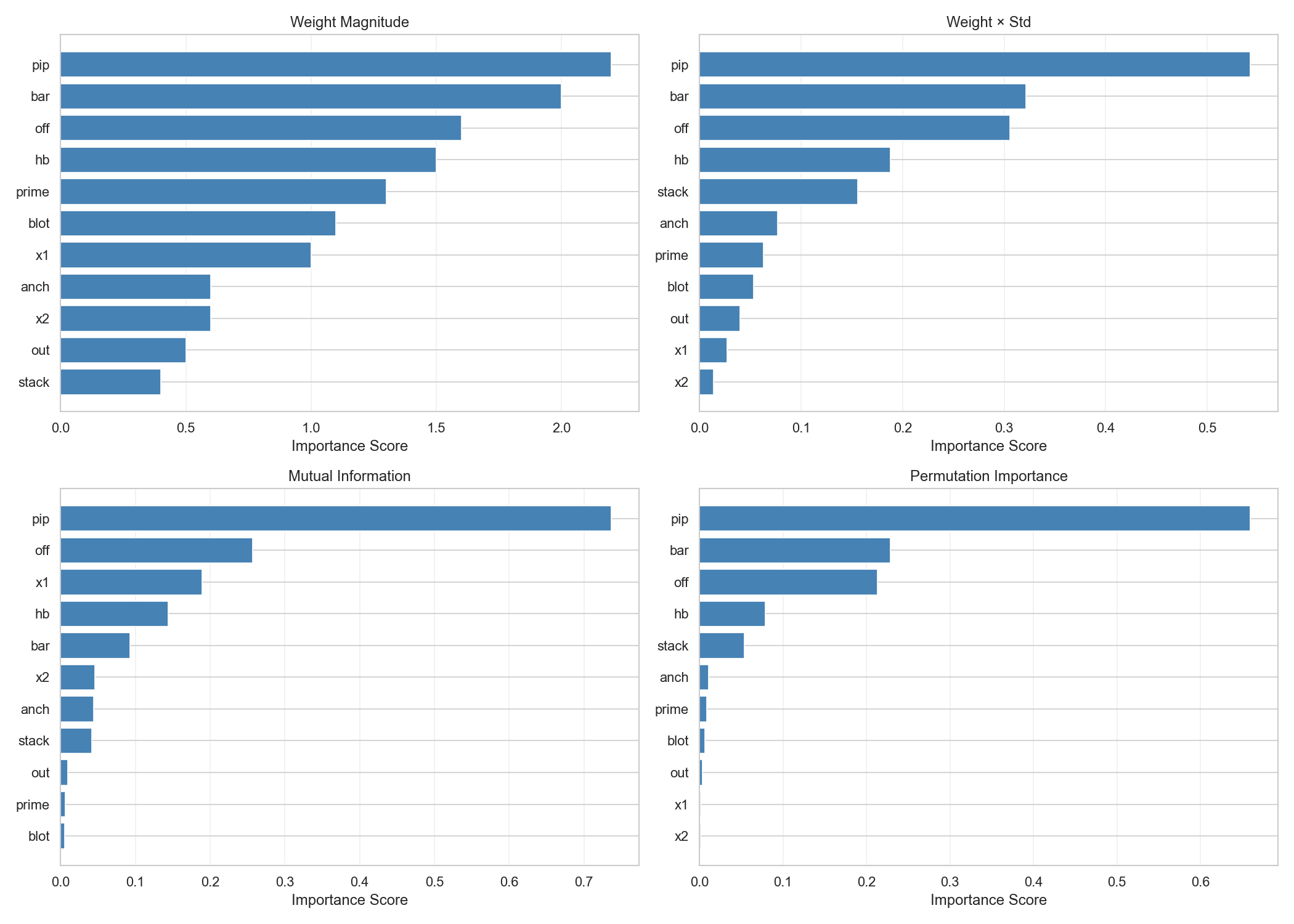
• Correlation matrix: IMG/bras_analysis_correlation.png
• Feature importance: IMG/bras_analysis_importance.png

More detailed set (10k samples) in ds_analysis/:

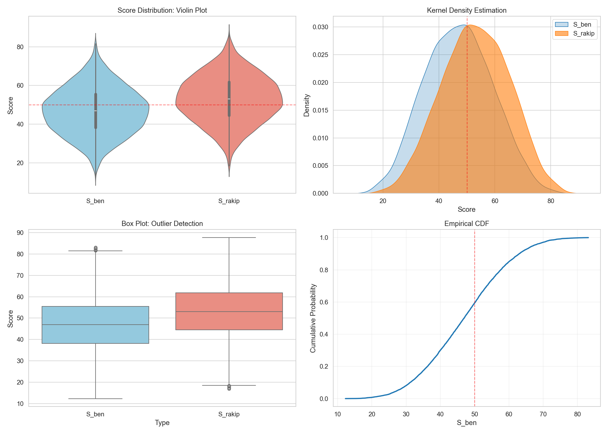
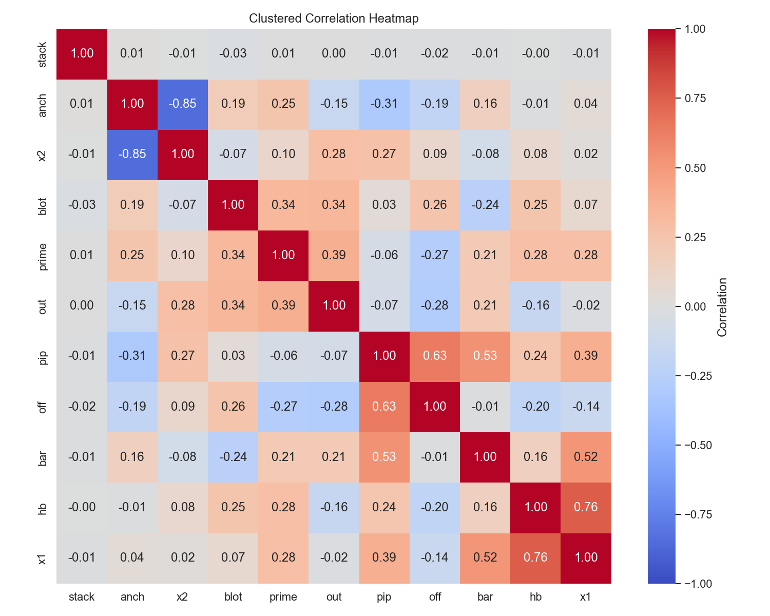
• Distributions: ds_analysis/01_score_distributions.png
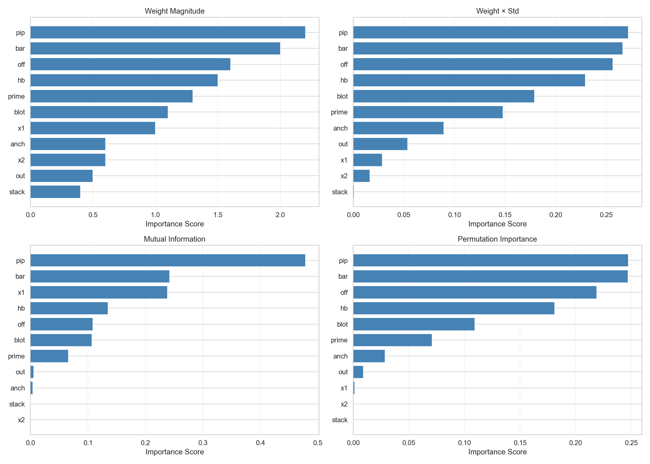
• Correlation (clustered): ds_analysis/04_correlation_clustered.png
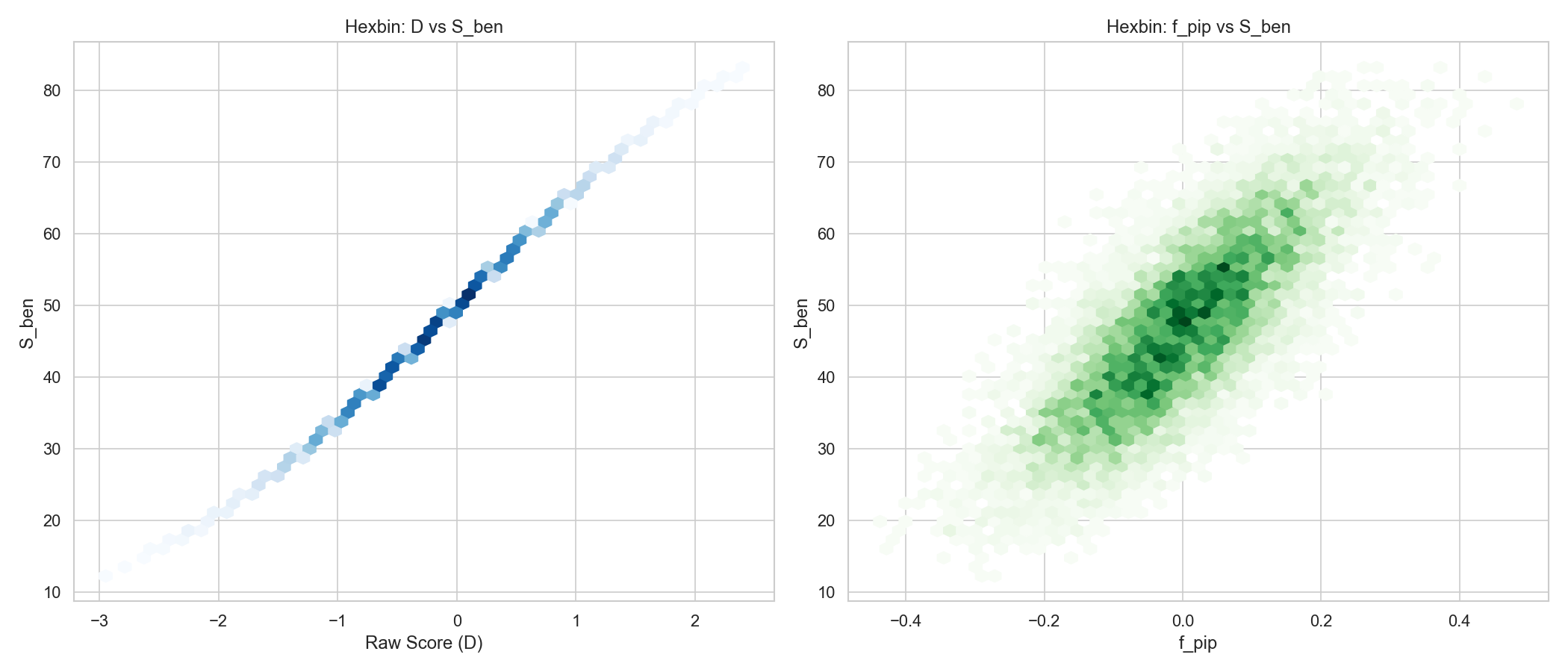
• Feature importance: ds_analysis/08_feature_importance.png
• Relationship hexbin: ds_analysis/05_hexbin_relationships.png

Related reports: docs/ras_whitepaper.md, docs/ras_verification_and_performance.md.

Doubling (Cube) Insights

We want smooth, symmetric, and threshold-sensitive behavior for doubling. Since g(D)=tanh(D/σ) is a single function, this is naturally achieved.

Short findings (ds_analysis_doubling2/dataset.csv):

• E[p] ≈ 0.500, std ≈ 0.145 (close to balanced)
• S_me means by D range: [-0.5,0.0]→~45.8, [0.0,0.5]→~54.1, [1.0,1.5]→~69.2, [2.0,2.5]→~81.0
• Thus, S_me rises smoothly and monotonically with D; drop/take windows separate cleanly
• By symmetry, opponent's perspective is automatic: S_op = 100 − S_me

Key visuals (doubling focus):

• ds_analysis_doubling2/01_score_distributions.png
• ds_analysis_doubling2/07_statistical_tests.png
• ds_analysis_doubling2/08_feature_importance.png

Speed, Cost, and Engineering

• ~0.78 ms/position (single core) → suitable for real-time engines
• Light dependencies; easily portable with NumPy
• Features are modular; weight calibration can be domain-expert guided

Reproduction

• Basic tests: python test_bras.py
• Quick analysis & visuals: python analyze_bras.py.py
• Data science pipeline (parameterized):
  • python data_science_analysis.py --n-samples 8000 --output-dir ds_analysis_doubling2

Quick mathematical check (antisymmetry & transform):

python -c "import pandas as pd, numpy as np; df=pd.read_csv('ds_analysis_doubling2/dataset.csv'); \
print(np.abs(df['S_me']+df['S_op']-100).max()); \
print(np.abs((df['S_me']-50)/50 - np.tanh(df['D']/3)).max())"

Closing

With an antisymmetric, interpretable, and closed-form evaluation function, we have a fast, robust, and practical foundation for Backgammon. This provides a strong “pre-evaluator” for search/simulation and, on its own, makes a practical heuristic for mobile/edge deployment. The cube decisions benefit from smooth, symmetric thresholds. With new data, the weights can be fine-tuned and confidently recalibrated with the same analysis/test suite.

—

Sources and Code:

• Mathematics: docs/ras_mathematical_foundations.md
• Academic report: docs/ras_whitepaper.md
• Analysis report: docs/ras_verification_and_performance.md
• Implementation: bras_evaluator.py
• Test suite: test_bras.py
• Analyses: analyze_bras.py.py, data_science_analysis.py

---

In-Depth Explanation: From Design to Validation

This section is the longer version, where I answer "why, how, when" in detail, explaining design decisions and the validation process. Can be read like a blog series; skip between sections as needed.

1) Problem Nucleus: Speed, Interpretability, Mathematical Guarantees

Backgammon, while laden with dice uncertainty, still has regular position patterns: pip balance, bar disadvantage, home board power, prime and anchor architecture, blot risk, midboard control, etc. Two industry strategies dominate:

• “Heavy but nonlinear” approaches: Monte Carlo simulations, tree search.
• “Light and interpretable” approaches: Feature-based heuristics.

My aim is to combine the best of both: Single-pass, explainable, mathematically robust; mobile/edge speed, reportable consistency, calibratable with new data.

2) Design Principles and Constraints

• Must be antisymmetric: When you flip color/board, scores swap (neutrality, logical soundness)
• Bounded output: S ∈ [0,100]; easy for human-centric interpretation (percentile intuition)
• Monotonic and smooth: Advantage in pip↑ → S_me↑, bar disadvantage↑ → S_me↓; smooth throughout
• Interpretable features: Each f_i should represent real game intuition, be normalized
• Closed form & performance: Single pass computation; vectorized, fast

3) Feature Design: The Nuances of the f_i

Here each feature's game logic and normalization rationale are presented. Full definitions and denominators in docs/ras_mathematical_foundations.md.

• Pip (f_pip): Total pip count difference; denominator 375 assures within bounds. See bras_evaluator.py:116.
• Bar (f_bar): Difference in checkers on the bar. Very penalizing since it kills short-term freedom. Code: bras_evaluator.py:179.
• Off (f_off): Bear-off progress, endgame fuel. Code: bras_evaluator.py:187.
• Home Board (f_hb): Closed points (1–6); proxy for jailing strength post-hit. Code: bras_evaluator.py:132.
• Prime (f_prime): Longest closed run (max 6); restricts movement. Code: bras_evaluator.py:149 + helper _longest_run at bras_evaluator.py:157.
• Anchor (f_anch): Secure points in opponent's home, reduces getting closed out/gammoned. Code: bras_evaluator.py:170.
• Blot (f_blot): Open checker penalties, regionally weighted by ρ(i); home>mid>opp.home (1.5 / 1.0 / 1.2). Code: bras_evaluator.py:196, 100.
• Stack (f_stack): >5 checker stack penalty (flexibility loss). Code: bras_evaluator.py:206.
• Out (f_out): Control over midboard (7–18 corridor). Code: bras_evaluator.py:195.
• Interaction 1 (f_x1): Home power × opponent's bar; strong home punishes opponent on bar more. Code: bras_evaluator.py:221.
• Interaction 2 (f_x2): Prime × opponent's anchor, counters primes somewhat, negative weight. Code: bras_evaluator.py:233.

Normalization (denominators) serves: (1) Features can be summed on same scale; (2) Weight reflects direct impact on the score.

4) Weights and Calibration Rationale

Initial weights are expert-driven, then pass a “checklist” data pass:

• "Bar is a heavy disadvantage" → w_bar = 2.0
• "Pip matters in all phases" → w_pip = 2.2
• "Measuring endgame speed matters" → w_off = 1.6
• "Home board and prime are important but not extremes" → w_hb = 1.5, w_prime = 1.3
• "Blot is always risky: mid-level" → w_blot = 1.1
• "Midboard support" → w_out = 0.5
• "Anchor is a safe haven" → w_anch = 0.6
• "Stacking is rare but harmful" → w_stack = 0.4
• "Interactions" → w_x1 = 1.0, w_x2 = -0.6

After data, ranking by |w|·std; practically, pip, bar, off, blot dominate (see plots and tables).

5) Transformation Function: Why tanh, Why σ=3?

tanh is naturally odd, i.e., g(-x)=-g(x), making it ideal for antisymmetric design. Bounded to [-1,1], smooth in center, well-behaved derivative. σ=3 calibration achieves:

• Typical D in [-3,3], so score band is ~50±38; extremes separated but not oversaturated
• Most random positions sit near tanh’s linear region, no over-saturation

Logistic also considered, but tanh + affine map (50±50·g) is cleaner for centering and symmetry.

6) Antisymmetry: Guaranteed by Operator

Flip operator: Ŷ_i := O_{25−i}, Ô_i := Y_{25−i}, b_Y↔b_O, y_Y↔y_O. This flips all feature signs → f_i(tilde) = −f_i. Hence D(tilde) = −D, S_me(tilde) = 100 − S_me. In implementation: bras_evaluator.py:306.

7) Monotonicity: A Small Derivative Tour

From the doc, for pip:

∂S_me/∂R = 50·g’(D)·w_pip/375 = 50·w_pip/(375·σ)·sech²(D/σ) > 0

Bar increase for me is bad → ∂S_me/∂b_Y < 0. This is scenario tested in test_bras.py:303.

8) Implementation Notes & Performance

Key code choices:

• Vectorized ops (NumPy) for ~0.78 ms/position. See: generation loop in analyze_bras.py.py.
• _longest_run computes prime length via linear scan with early break and small buffer.
• rho(i) and rho_star(i) encode location-dependent blot risk (home, mid, opp.home), integrating “point risk isn’t uniform” into the game.

9) Test Suite: How I Broke and Fixed It

Tests in test_bras.py cover five axes:

1. Antisymmetry: Total=100 and matching after flip (N=1000). Max error ~1e−14. (test_bras.py:139)
2. Documentation examples: Opening 50.000, contact ex: S≈47.893, D≈−0.1265. (test_bras.py:192)
3. Feature bounds: f_i ∈ [-1,1] checked, no violations. (test_bras.py:240)
4. Score bounds: S ∈ [0,100] checked, no violations. (test_bras.py:274)
5. Monotonicity: Pip↑ ⇒ S_me↑, My bar↑ ⇒ S_me↓. (test_bras.py:303)
6. Edge cases: All bar, all off, max stack. (test_bras.py:402)

Random generator focuses on certain points (to increase stack frequency), see: test_bras.py:467.

10) Statistical Analysis & Visuals

Two layers of reports:

• Fast general set (analyze_bras.py.py): summarizing score, D, transform, and antisymmetry
• Data science set (data_science_analysis.py): EDA, correlation, importance, VIF, dimensionality reduction, clustering, sensitivity

Sample visuals (general):

Detailed set (10k samples, ds_analysis/):

Summary: Score mean ~46.9 (slight disadvantage bias in generator), std ~12.1; D mean ~−0.20, std ~0.77. Most significant features: pip, bar, off, blot; correlations mostly as expected (pip–off, hb–x1).

11) Doubling (Cube): Windows, Thresholds, Smoothness

Doubling is thresholded by nature; g(D)=tanh(D/σ) makes this transition smooth. From ds_analysis_doubling2/dataset.csv:

• E[p]≈0.500, std≈0.145.
• D intervals: [-0.5,0.0]→S≈45.8, [0.0,0.5]→S≈54.1, [1.0,1.5]→S≈69.2, [2.0,2.5]→S≈81.0.
• Symmetry: Opponent’s side flips naturally: S_op=100−S_me.

This cleanly splits “initial double” and “drop” regions. Surface is also uniform, does not jump with small noise.

Doubling visuals (samples):

12) Limitations & Future Work

• Handcrafted features help interpretability, but aren't aiming for neural net raw accuracy ceiling. Hybrid (this + small NN) could be next.
• Weights static; phase-aware adaptive weighting (phase detector) could add value.
• Generated distribution can be re-calibrated with real game data, adjusting w and σ.
• Blot's regional weights can be personalized for player style.

13) Quick Usage & Reproduction

Basic tests:

python test_bras.py

Quick analysis and visuals:

python analyze_bras.py.py

Data science pipeline (with parameters):

python data_science_analysis.py --n-samples 8000 --output-dir ds_analysis_doubling2

Quick math validation:

python -c "import pandas as pd, numpy as np; df=pd.read_csv('ds_analysis_doubling2/dataset.csv'); \
print(np.abs(df['S_me']+df['S_op']-100).max()); \
print(np.abs((df['S_me']-50)/50 - np.tanh(df['D']/3)).max())"

14) Mini Code Example

import numpy as np
from tavla_evaluator import TavlaEvaluator, create_opening_position

e = TavlaEvaluator()
pos = create_opening_position()
S_me, S_op = e.compute_score(pos)
print(S_me, S_op)

# Detailed output
detail = e.evaluate_detailed(pos)
print(detail['features'])
print(detail['D'], detail['g'])

15) Final Words

A good evaluation function isn’t so much “correct” as it is “consistent and useful.” This approach balances speed/fidelity/interpretability for Backgammon. It smooths the cube decision surface, gives a robust prior for search/simulation, and serves as a practical heuristic by itself for mobile/edge. Very receptive to improvement with feedback and new data.