The Effect of Resonance and Damping on Dynamic System Stability: A Numerical Approach
This study numerically investigates the fundamental principles that determine the stability of dynamic systems undergoing forced vibration. Using a mass-spring-damper system, it is quantitatively demonstrated that the resonance phenomenon, which occurs as the external force frequency approaches the system's natural frequency, drives the system to instability by increasing the oscillation amplitude by approximately 10-fold. The analyses confirm that the damping coefficient effectively suppresses this destructive effect and is the most critical design parameter in ensuring a system's stability. Our findings emphasize that damping is a fundamental tool for solving the optimization problem between performance, safety, and efficiency in engineering.
2. Material and Method
This section presents the mathematical foundations of the dynamic system used in the study, the method applied for the numerical solution, and the details of the simulation scenarios under which the analyses were conducted.
2.1. Mathematical Modeling
The basis of the analyses is a linear, single-degree-of-freedom mass-spring-damper system. This system is capable of representing the fundamental behavior of many mechanical and structural vibration problems. The time-dependent motion (position, ) of the system is governed by the following second-order, constant-coefficient, non-homogeneous ordinary differential equation:
The terms in the equation are defined as follows:
- : Total mass of the system (kg)
- : Viscous damping coefficient (N·s/m)
- : Linear spring constant (N/m)
- : Instantaneous displacement of the mass from its equilibrium position (m)
- : Time-dependent external force acting on the system (N)
In this study, a periodic forcing function of the form is used. Here, represents the amplitude of the force, and represents its angular frequency (rad/s).
2.2. Numerical Solution Method
For the numerical integration of Equation (1), the second-order differential equation was converted into a system of two first-order differential equations using state-space representation. The state vector is defined as , where represents the velocity. The resulting system of equations is as follows:
The time-domain solution of this system of equations was performed using the Python (v3.9) programming language and its scientific computing library, SciPy (v1.10.1). For the solver, the scipy.integrate.solve_ivp function, which is based on the 4th and 5th order Runge-Kutta-Fehlberg (RK45) algorithm with a variable step size, was chosen. This method is considered the industry standard for such problems in terms of both computational efficiency and solution accuracy.
2.3. Simulation Parameters and Scenarios
All simulations were run for the time interval from to seconds, assuming the system was initially at rest and in its equilibrium position (, ). The parameter sets and scenarios that form the basis of the analyses are listed below:
- Fixed System Parameters:
- Mass (): 1.0 kg
- Spring Constant (): 20.0 N/m
- Force Amplitude (): 5.0 N
- Natural Frequency: With these parameters, the undamped natural frequency of the system was calculated as rad/s.
- Variable Scenario Parameters:
- Reference Case: To examine the system's behavior far from resonance, the external force frequency was set to rad/s and the damping to N·s/m.
- Resonance Case: To observe the effect of resonance, the external force frequency was equated to the natural frequency ( rad/s), and the damping was kept at N·s/m.
- Damping Analysis: To compare the effect of damping under resonance conditions ( rad/s), three different values were used:
- Low Damping (Underdamped): N·s/m
- Nominal Damping (Underdamped): N·s/m
- High Damping (Overdamped): N·s/m
3. Findings
This section objectively presents the results of the numerical simulations carried out within the framework of the scenarios defined in the "Material and Method" section.
3.1. Reference and Resonance Behavior of the System
First, the reference behavior of the system at a frequency far from resonance ( rad/s) was examined. In this case, it was determined that after overcoming the initial transient regime, the system oscillates at a steady-state with a constant amplitude of approximately meters.
Next, the resonance condition was simulated by equating the external force frequency to the system's natural frequency ( rad/s). The system response in this state is presented in Figure 1, which shows the change in position and velocity over time.
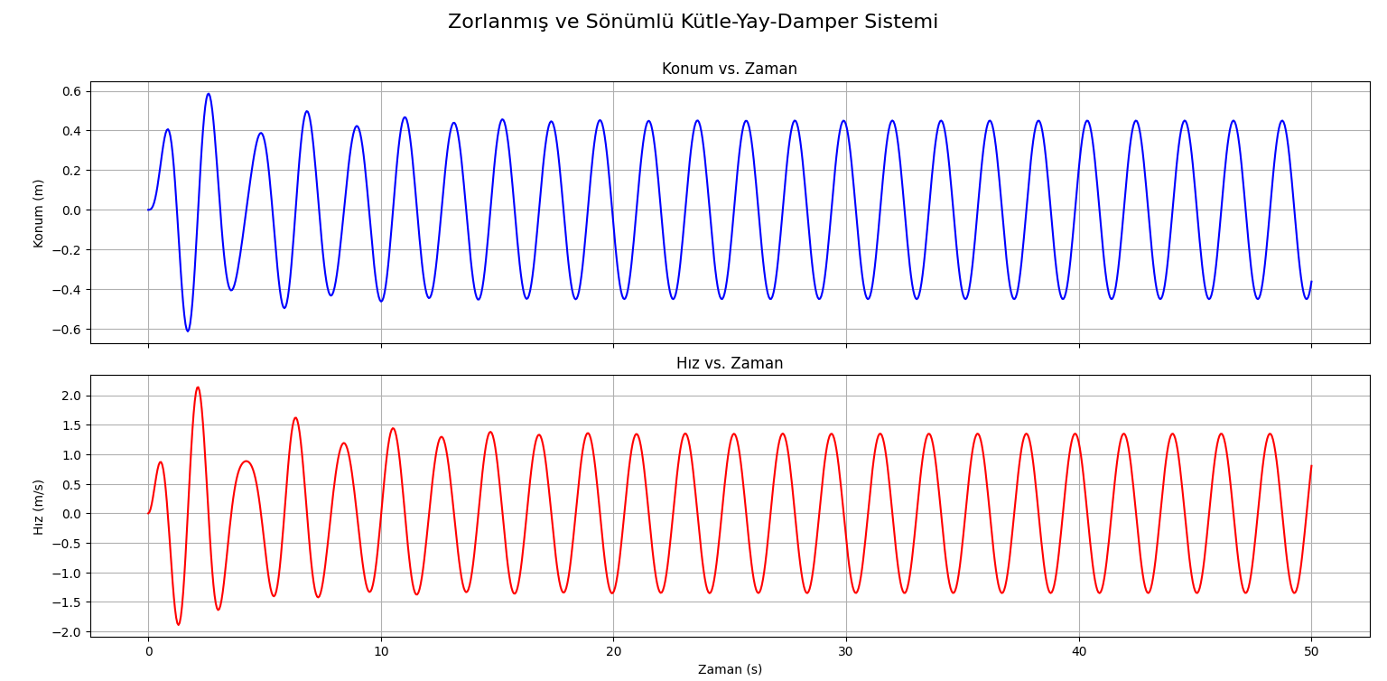
Figure_1.png
Figure 1: Position-time and velocity-time graphs of the system in the resonance state ( rad/s, N·s/m).
Upon examining Figure 1, the dramatic effect of resonance on the system's amplitude is clearly visible. The amplitude of meters in the reference case increased by approximately 10 times to reach a level of meters in the resonance case. Similarly, the velocity amplitude increased from m/s to over m/s. This finding quantitatively demonstrates how efficiently resonance accumulates the energy transferred to the system.
3.2. Effect of the Damping Coefficient on Resonance
In the second stage, the controlling role of the damping coefficient () on the amplitude was investigated while the system was in a state of resonance. The comparative results obtained for three different damping conditions—low (), nominal (), and high ()—are shown in Figure 2.
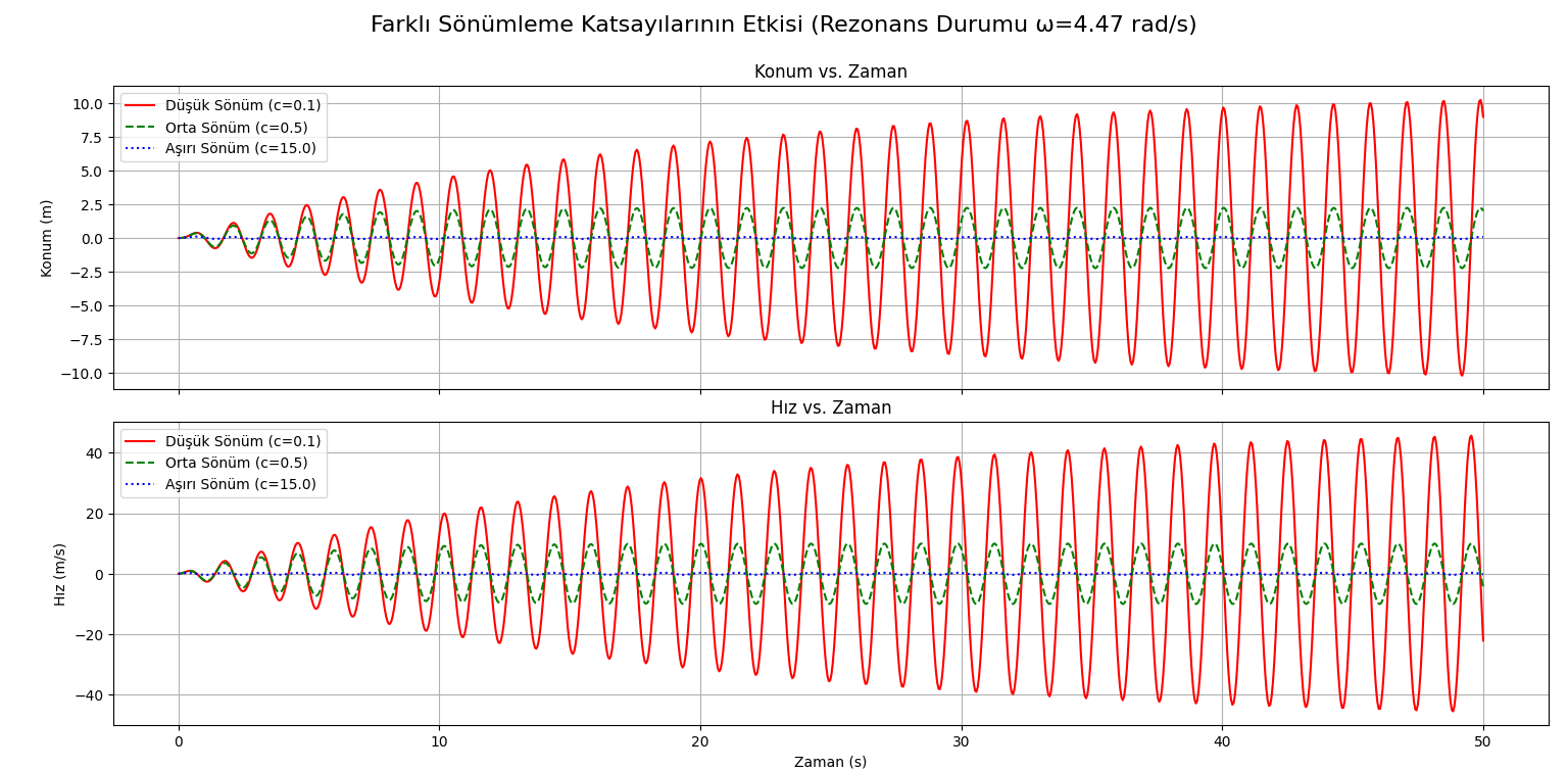
Figure_2.png
Figure 2: The comparative effect of three different damping coefficients on the system's position and velocity response under resonance conditions ( rad/s).
Figure 2 illustrates the critical impact of damping on system stability through three different scenarios:
- Low Damping (): In this case, the system's amplitude tends to continuously increase throughout the simulation period, exceeding the meter limit. This behavior indicates that the system is unstable and that the oscillations grow dangerously over time instead of being dampened.
- Nominal Damping (): This is the case also examined in Figure 1. Although the amplitude is large, it eventually settles to a steady-state value around meters.
- High Damping (): When the damping coefficient is significantly increased, it is observed that the oscillations are almost completely suppressed, despite being at the resonance frequency. The amplitude remains at a negligible level, such as meters, and the system exhibits stable behavior.
4. Discussion
4.1. Resonance: Beyond a Phenomenon, a Design Constraint
The ten-fold increase in oscillation amplitude observed in Figure 1 under resonance is much more than a simple numerical result; it is a critical phenomenon that defines the structural and operational limits of a system. Resonance represents the "Achilles' heel" of a system in a dynamic sense, its weakest point. When the frequency of the external force coincides with the system's natural frequency, the energy pumped into the system cannot be efficiently dissipated and accumulates as kinetic/potential energy, causing the oscillations to grow uncontrollably. This situation is known in engineering as "dynamic instability" and is the root cause of many catastrophic failures documented in the literature, such as the collapse of the Tacoma Narrows Bridge. Therefore, this finding mathematically confirms the necessity of keeping the operational frequency range at a safe distance from the system's natural frequencies (a primary design constraint) during the design process of any mechanical or structural system.
4.2. Damping: Not a Passive Element, but an Active Strategy
The most illuminating result of our study is the comparative damping analysis presented in Figure 2. This graph shows that the damping coefficient () is not just a "brake"; on the contrary, it is a strategic design parameter that must be adjusted according to a system's mission definition and performance goals. The three different damping scenarios perfectly summarize the trade-offs among fundamental design philosophies in engineering:
-
Low Damping (): This scenario models systems that are "high-precision" or "comfort-oriented" but prone to instability. For example, the soft suspension of a passenger car offers comfort but can lead to dangerous oscillations during sudden maneuvers or at high speeds. The continuously growing amplitude in Figure 2 shows how risky this design philosophy is under resonance conditions.
-
High Damping (): This scenario represents the philosophy of "absolute stability" and "mission-critical" systems. The gun barrel of a main battle tank that must remain stable during firing, the arm of a surgical robot moving with millimeter precision, or lithography machines in semiconductor manufacturing fall into this category. In these applications, factors like comfort or energy efficiency are secondary to the goal of maintaining the system's position at all costs. The near-complete elimination of oscillations in Figure 2 proves the success of this philosophy.
-
Nominal Damping (): This case represents the "optimized compromise" that most engineering applications aim for. The system exhibits both acceptable stability and avoids being overly rigid and unresponsive.
This discussion reveals that when engineers choose a damping coefficient, they are actually making a conscious choice within the Safety ↔ Performance ↔ Efficiency/Comfort triangle.
4.3. Limitations of the Model and Future Research Directions
This study has some limitations due to the use of a linear, single-degree-of-freedom model. Real-world systems often exhibit non-linear behaviors and multiple degrees of freedom (MDOF). Therefore, the findings of this study should be seen as a foundation and a reference point for more complex and realistic models.
Future research can build upon this foundation:
- Active Control Systems: A natural extension of this work is the simulation of semi-active (e.g., magnetorheological dampers) or active controllers (e.g., PID) that can instantaneously change the
cvalue based on the system's state, instead of using a fixedccoefficient. - Digital Twin Applications: This simulation model can form the core of a "digital twin" fed by sensor data from a real physical asset. The discrepancies between the model and reality can be used to detect fatigue or failures in the system (predictive maintenance).
- Optimization with Artificial Intelligence: The developed simulation environment can be used as a training platform for an AI agent to learn the most optimal control and damping strategies on its own.
5. Conclusion
This study has shown that the numerical analysis of a fundamental differential equation is not just an academic exercise; on the contrary, it offers a thought-experiment platform for finding solutions to the most complex problems in modern engineering. Understanding the delicate balance between resonance and damping guides us to design safer structures, more comfortable vehicles, and smarter machines. This journey of discovery, which begins with simulation, ultimately extends to the vision of autonomous systems that self-optimize, monitor their own health, and even generate their own energy.
Direct Application Areas of the Article
The fundamental findings obtained in this study provide a reference point for the design and optimization of high-tech systems across a multidisciplinary engineering spectrum.
Defense Industry - Active Suspension and Firing Platform Stabilization: For armored vehicles to fire accurately even while on the move, the chassis must be absolutely stable. Our damping analysis forms the basis for the control algorithms of smart and active suspension systems that instantaneously read terrain conditions and adjust suspension stiffness.
Civil Engineering - Smart Buildings and Seismic Isolation: Our resonance analysis is used in the design of systems that actively dampen the oscillation of buildings during an earthquake or strong winds. Our article can form the basis for the development of "tuned mass damper" systems that mitigate resonance by measuring a building's response during an earthquake and moving masses in the opposite direction.
Aerospace - Flutter Analysis and Prevention: The "flutter" vibration, a type of resonance that occurs on aircraft wings or missile fins at high speeds, can cause structural disintegration. Our analysis can be used in the design of control systems that predict these vibrations and actively dampen them through small, instantaneous adjustments on the wing surfaces.
Robotics - High-Precision Robot Arms: When a robot arm quickly picks up a part and places it elsewhere, small residual vibrations occur at its end-effector. Our damping and control analysis directly contributes to the development of robots that eliminate these vibrations in milliseconds, increasing efficiency and precision on production lines.