1. Blog
  2. Static Positional Evaluation (SPE)
Back to Articles

Static Positional Evaluation (SPE)

August 26, 2025
1609 words
9 min read
#backgammon algorithm#backgammon strategy#heuristic evaluation#bar entry probability

A New Checker‑Combination Scoring Formula

Author: Umutcan EDIZASLAN Version: 1.0 Date: August 26, 2025

Abstract

Backgammon evaluation often blends race metrics with contact-position heuristics. I introduce Static Positional Evaluation (SPE), a succinct and rigorous checker-combination formula that outputs an interpretable, bounded score on [0, 100]. By construction, 50 denotes equality, and the mapping is smooth and saturates at extremes, making it suitable for both human interpretation and downstream algorithms (e.g., move ranking, search pruning, educational tools).

1. Introduction

Backgammon evaluation often blends race metrics with contact‑position heuristics. I propose SPE, a succinct and rigorous checker‑combination formula that outputs an interpretable, bounded score on [0, 100]. By construction, 50 denotes equality, and the mapping is smooth and saturates at extremes, suitable for both human interpretation and downstream algorithms (e.g., move ranking, search pruning, or educational tools).


2. Notation and Scoring Overview

2.1 Board & counts

  • Points numbered 1..24 from your home board (1..6) outward; 24 is farthest from your home.
  • nX(j)n_X(j)nX​(j): number of checkers for side X∈{You,Opp}X\in\{\mathrm{You},\mathrm{Opp}\}X∈{You,Opp} on point jjj.
  • bXb_XbX​: number of XXX’s checkers on the bar.
  • A point is closed for XXX if nX(j)≥2n_X(j)\ge 2nX​(j)≥2.
  • Triangular number: Tri(ℓ)=ℓ(ℓ+1)/2\mathrm{Tri}(\ell)=\ell(\ell+1)/2Tri(ℓ)=ℓ(ℓ+1)/2.

Pip counts (to each side’s own home):

PYou=∑j=124j nYou(j)+25 bYou,POpp=∑j=124(25−j) nOpp(j)+25 bOpp.P_{\text{You}}=\sum_{j=1}^{24} j\,n_{\text{You}}(j)+25\,b_{\text{You}},\qquad P_{\text{Opp}}=\sum_{j=1}^{24} (25-j)\,n_{\text{Opp}}(j)+25\,b_{\text{Opp}}.PYou​=j=1∑24​jnYou​(j)+25bYou​,POpp​=j=1∑24​(25−j)nOpp​(j)+25bOpp​.

This symmetric definition measures distance to each side’s bear‑off.

> Image (Figure 1) here helps orientation.


2.2 Features (checker‑combination terms)

All features are computed for You and Opponent, then combined as net advantages Δ(⋅)=You−Opp\Delta(\cdot)=\text{You}-\text{Opp}Δ(⋅)=You−Opp, with sign flips where appropriate.

  1. Race (normalized pip advantage):
R=POpp−PYou167.R=\frac{P_{\text{Opp}}-P_{\text{You}}}{167}.R=167POpp​−PYou​​.
  1. Home‑board made points (1..6 / 24..19):
HBX=∑k=16hk 1[nX(k)≥2]for You,HB_X=\sum_{k=1}^{6} h_k\,\mathbf{1}[n_X(k)\ge 2]\quad\text{for You},HBX​=k=1∑6​hk​1[nX​(k)≥2]for You,

and symmetrically for Opp (mapping 24→1, 23→2, …, 19→6). Default weights: (h1,…,h6)=(0.30,0.45,0.60,0.95,1.20,0.80)(h_1,\dots,h_6)=(0.30,0.45,0.60,0.95,1.20,0.80)(h1​,…,h6​)=(0.30,0.45,0.60,0.95,1.20,0.80).

  1. Prime strength (consecutive closed points): Let HYou={1,…,6}H_{\text{You}}=\{1,\dots,6\}HYou​={1,…,6}, OYou={7,…,12}O_{\text{You}}=\{7,\dots,12\}OYou​={7,…,12} and for Opp HOpp={24,…,19}H_{\text{Opp}}=\{24,\dots,19\}HOpp​={24,…,19}, OOpp={18,…,13}O_{\text{Opp}}=\{18,\dots,13\}OOpp​={18,…,13}. For each region, sum Tri(ℓ)\mathrm{Tri}(\ell)Tri(ℓ) over maximal runs of closed points; e.g.,
PRhome,X=∑iTri(ℓi(H)),PRouter,X=∑iTri(ℓi(O)).PR_{\text{home},X}=\sum_{i}\mathrm{Tri}(\ell_i^{(H)}),\qquad PR_{\text{outer},X}=\sum_{i}\mathrm{Tri}(\ell_i^{(O)}).PRhome,X​=i∑​Tri(ℓi(H)​),PRouter,X​=i∑​Tri(ℓi(O)​).
  1. Anchors in the opponent’s home board:
ANYou=∑j=1924aj 1[nYou(j)≥2],ANOpp=∑j=16a25−j 1[nOpp(j)≥2].AN_{\text{You}}=\sum_{j=19}^{24} a_j\,\mathbf{1}[n_{\text{You}}(j)\ge 2],\quad AN_{\text{Opp}}=\sum_{j=1}^{6} a_{25-j}\,\mathbf{1}[n_{\text{Opp}}(j)\ge 2].ANYou​=j=19∑24​aj​1[nYou​(j)≥2],ANOpp​=j=1∑6​a25−j​1[nOpp​(j)≥2].

Default (a24,a23,a22,a21,a20,a19)=(0.50,0.65,0.85,1.05,1.25,0.90)(a_{24},a_{23},a_{22},a_{21},a_{20},a_{19})=(0.50,0.65,0.85,1.05,1.25,0.90)(a24​,a23​,a22​,a21​,a20​,a19​)=(0.50,0.65,0.85,1.05,1.25,0.90).

  1. Immediate shots next roll (approximation): For each blot (exactly one checker) at point jjj, collect distinct hitting distances available to the attacker next roll:
  • If You attack: distances d=i−jd=i-jd=i−j with i∈{j+1,…,min⁡(j+6,24)}i\in\{j+1,\dots,\min(j+6,24)\}i∈{j+1,…,min(j+6,24)} where nYou(i)≥1n_{\text{You}}(i)\ge 1nYou​(i)≥1.
  • If Opp attack: distances d=j−id=j-id=j−i with i∈{max⁡(1,j−6),…,j−1}i\in\{\max(1,j-6),\dots,j-1\}i∈{max(1,j−6),…,j−1} where nOpp(i)≥1n_{\text{Opp}}(i)\ge 1nOpp​(i)≥1.

Let mmm be the number of distinct distances; approximate:

p(m)=1−(6−m6)2(m=0..6;  p=1136,2036,2736,3236,3536,1 for m=1..6).p(m)=1-\Big(\frac{6-m}{6}\Big)^2 \quad(m=0..6;\; p=\tfrac{11}{36},\tfrac{20}{36},\tfrac{27}{36},\tfrac{32}{36},\tfrac{35}{36},1\ \text{for }m=1..6).p(m)=1−(66−m​)2(m=0..6;p=3611​,3620​,3627​,3632​,3635​,1 for m=1..6).

Sum p(m)p(m)p(m) over all enemy blots to get SHXSH_XSHX​.

  1. Entry difficulty (bar vs closed home points): Let cXc_XcX​ be the count of opponent closed points in the home board you must enter against. Approximate “fail to enter” as (c/6)2(c/6)^2(c/6)2:
ENX=bX(cX6)2.EN_X=b_X\Big(\frac{c_X}{6}\Big)^2.ENX​=bX​(6cX​​)2.

I use ΔEN=ENOpp−ENYou\Delta EN=EN_{\text{Opp}}-EN_{\text{You}}ΔEN=ENOpp​−ENYou​ so higher is good for you.

  1. Flexibility / builders (spares beyond two, capped at two):
FLYou=∑j=713 ⁣min⁡(max⁡(n−2,0),2)  +  12∑j=1418 ⁣min⁡(max⁡(n−2,0),2),FL_{\text{You}}=\sum_{j=7}^{13}\!\min(\max(n-2,0),2)\;+\;\tfrac{1}{2}\sum_{j=14}^{18}\!\min(\max(n-2,0),2),FLYou​=j=7∑13​min(max(n−2,0),2)+21​j=14∑18​min(max(n−2,0),2), FLOpp=∑j=1218 ⁣min⁡(max⁡(n−2,0),2)  +  12∑j=711 ⁣min⁡(max⁡(n−2,0),2).FL_{\text{Opp}}=\sum_{j=12}^{18}\!\min(\max(n-2,0),2)\;+\;\tfrac{1}{2}\sum_{j=7}^{11}\!\min(\max(n-2,0),2).FLOpp​=j=12∑18​min(max(n−2,0),2)+21​j=7∑11​min(max(n−2,0),2).
  1. Stack penalty (option‑limiting stacks):
STX=∑j=124max⁡(nX(j)−4, 0),ΔST=STOpp−STYou.ST_X=\sum_{j=1}^{24}\max(n_X(j)-4,\,0),\quad \Delta ST=ST_{\text{Opp}}-ST_{\text{You}}.STX​=j=1∑24​max(nX​(j)−4,0),ΔST=STOpp​−STYou​.
  1. Back men liability (farthest stragglers): For You (farthest are 24,23,22):
BKYou=1.0 n(24)+0.7 n(23)+0.4 n(22).BK_{\text{You}}=1.0\,n(24)+0.7\,n(23)+0.4\,n(22).BKYou​=1.0n(24)+0.7n(23)+0.4n(22).

For Opp (farthest are 1,2,3):

BKOpp=1.0 n(1)+0.7 n(2)+0.4 n(3),BK_{\text{Opp}}=1.0\,n(1)+0.7\,n(2)+0.4\,n(3),BKOpp​=1.0n(1)+0.7n(2)+0.4n(3),

then ΔBK=BKOpp−BKYou\Delta BK=BK_{\text{Opp}}-BK_{\text{You}}ΔBK=BKOpp​−BKYou​ so higher is good for you.

> Image (Figure 2) can call out these regions and features.


2.3 One‑line SPE equation

  SPE  =  50+50 tanh⁡ ⁣(Dσ)  \boxed{\;\text{SPE} \;=\; 50 + 50\,\tanh\!\Big(\frac{D}{\sigma}\Big)\;}SPE=50+50tanh(σD​)​

with structural advantage

Damp;=wr R+whb ΔHB+wprh ΔPRhome+wpro ΔPRouter+wan ΔANamp;+wsh ΔSH+wen ΔEN+wfl ΔFL+wst ΔST+wbk ΔBK.\begin{aligned} D &= w_r\,R + w_{hb}\,\Delta HB + w_{prh}\,\Delta PR_{\text{home}} + w_{pro}\,\Delta PR_{\text{outer}} + w_{an}\,\Delta AN \\&\quad + w_{sh}\,\Delta SH + w_{en}\,\Delta EN + w_{fl}\,\Delta FL + w_{st}\,\Delta ST + w_{bk}\,\Delta BK. \end{aligned}D​amp;=wr​R+whb​ΔHB+wprh​ΔPRhome​+wpro​ΔPRouter​+wan​ΔANamp;+wsh​ΔSH+wen​ΔEN+wfl​ΔFL+wst​ΔST+wbk​ΔBK.​

2.4 Default weights and mapping scale

Termamp;wramp;whbamp;wprhamp;wproamp;wanamp;wshamp;wenamp;wflamp;wstamp;wbkValueamp;12.0amp;3.0amp;1.4amp;1.0amp;1.2amp;1.5amp;1.2amp;0.8amp;0.6amp;0.7σ=10.0.\begin{array}{l|cccccccccc} \text{Term} & w_r & w_{hb} & w_{prh} & w_{pro} & w_{an} & w_{sh} & w_{en} & w_{fl} & w_{st} & w_{bk} \\ \hline \text{Value} & 12.0 & 3.0 & 1.4 & 1.0 & 1.2 & 1.5 & 1.2 & 0.8 & 0.6 & 0.7 \end{array} \qquad \sigma=10.0.TermValue​amp;wr​amp;12.0​amp;whb​amp;3.0​amp;wprh​amp;1.4​amp;wpro​amp;1.0​amp;wan​amp;1.2​amp;wsh​amp;1.5​amp;wen​amp;1.2​amp;wfl​amp;0.8​amp;wst​amp;0.6​amp;wbk​amp;0.7​​σ=10.0.

> Image (Figure 3): include a simple plot of y=50+50tanh⁡(x/10)y=50+50\tanh(x/10)y=50+50tanh(x/10).


3. Mathematical Properties

Boundedness. Since ∣tanh⁡∣<1|\tanh|\lt 1∣tanh∣<1, SPE ∈(0,100)\in (0,100)∈(0,100); practically, it spans [0,100][0,100][0,100] by clamping.

Anti‑symmetry. Under the symmetric feature definitions above, the opponent’s advantage is −D-D−D. Hence:

SPEYou(D)+SPEOpp(−D)=100.\text{SPE}_{\text{You}}(D) + \text{SPE}_{\text{Opp}}(-D) = 100.SPEYou​(D)+SPEOpp​(−D)=100.

Continuity & robustness. Small feature changes yield small changes in DDD, smoothed by tanh⁡\tanhtanh.

Computational complexity. Each term scans at most 24 points: O(24)O(24)O(24) time and O(1)O(1)O(1) space.


4. Worked Example: Opening 6–6 (Bar‑Point Made)

Scenario. Standard starting layout. It’s your opening roll: 6‑6. I “use them to fill the 6‑point” in the standard sense:

24/18(2), 13/7(2)(bar‑point made at 7).\mathbf{24/18(2),\ 13/7(2)} \quad\text{(bar‑point made at 7)}.24/18(2), 13/7(2)(bar‑point made at 7).

Position after the move (your perspective):

  • You: 6(5), 7(2), 8(3), 13(3), 18(2). Bar = 0.
  • Opponent: 19(5), 17(3), 12(5), 1(2). Bar = 0.

> Image (Figure 4): show start and the resulting position.

I now compute each SPE term (defaults from §2.4).

4.1 Race RRR

PYou=6⋅5+7⋅2+8⋅3+13⋅3+18⋅2=143.P_{\text{You}}=6\cdot5+7\cdot2+8\cdot3+13\cdot3+18\cdot2=143.PYou​=6⋅5+7⋅2+8⋅3+13⋅3+18⋅2=143. POpp=(25 ⁣− ⁣19)⋅5+(25 ⁣− ⁣17)⋅3+(25 ⁣− ⁣12)⋅5+(25 ⁣− ⁣1)⋅2=6⋅5+8⋅3+13⋅5+24⋅2=167.P_{\text{Opp}}= (25\!-\!19)\cdot5+(25\!-\!17)\cdot3+(25\!-\!12)\cdot5+(25\!-\!1)\cdot2 =6\cdot5+8\cdot3+13\cdot5+24\cdot2=167.POpp​=(25−19)⋅5+(25−17)⋅3+(25−12)⋅5+(25−1)⋅2=6⋅5+8⋅3+13⋅5+24⋅2=167. R=167−143167=24167≈0.14371.R=\frac{167-143}{167}=\frac{24}{167}\approx 0.14371.R=167167−143​=16724​≈0.14371.

Contribution: wrR=12×0.14371=+1.7246w_r R = 12\times 0.14371 = \mathbf{+1.7246}wr​R=12×0.14371=+1.7246.

4.2 Home‑board points ΔHB\Delta HBΔHB

Both sides have only the 6‑point made in their home boards (h6=0.80)(h_6=0.80)(h6​=0.80) ⇒ ΔHB=0\Delta HB=0ΔHB=0. Contribution: 3.0×0=03.0\times 0=\mathbf{0}3.0×0=0.

4.3 Prime strength ΔPR\Delta PRΔPR

  • Your outer board has 7–8 closed (run length 2 ⇒ Tri(2)=3\mathrm{Tri}(2)=3Tri(2)=3).
  • Opponent’s outer board has 17 only (run length 1 ⇒ Tri(1)=1\mathrm{Tri}(1)=1Tri(1)=1). ΔPRouter=3−1=2\Delta PR_{\text{outer}}=3-1=2ΔPRouter​=3−1=2; ΔPRhome=0\Delta PR_{\text{home}}=0ΔPRhome​=0. Contribution: 1.0×2=+2.00001.0\times 2 = \mathbf{+2.0000}1.0×2=+2.0000 (outer), 1.4×0=01.4\times 0=\mathbf{0}1.4×0=0 (home).

4.4 Anchors ΔAN\Delta ANΔAN

You have no anchors in 19–24; Opponent has an anchor on your 1‑point (their 24): a24=0.50a_{24}=0.50a24​=0.50. ΔAN=−0.50\Delta AN=-0.50ΔAN=−0.50. Contribution: 1.2×(−0.50)=−0.60001.2\times(-0.50)=\mathbf{-0.6000}1.2×(−0.50)=−0.6000.

4.5 Immediate shots ΔSH\Delta SHΔSH

No blots ⇒ ΔSH=0\Delta SH=0ΔSH=0. Contribution: 0\mathbf{0}0.

4.6 Entry difficulty ΔEN\Delta ENΔEN

No one on the bar ⇒ ENYou=ENOpp=0EN_{\text{You}}=EN_{\text{Opp}}=0ENYou​=ENOpp​=0. Contribution: 0\mathbf{0}0.

4.7 Flexibility / builders ΔFL\Delta FLΔFL

  • You: spares beyond two at 8 (+1) and 13 (+1) ⇒ FLYou=2.0FL_{\text{You}}=2.0FLYou​=2.0.
  • Opp: 12 (+2), 17 (+1) ⇒ FLOpp=3.0FL_{\text{Opp}}=3.0FLOpp​=3.0. ΔFL=−1.0\Delta FL=-1.0ΔFL=−1.0. Contribution: 0.8×(−1.0)=−0.80000.8\times(-1.0)=\mathbf{-0.8000}0.8×(−1.0)=−0.8000.

4.8 Stack penalty ΔST\Delta STΔST

  • You: one stack of 5 at 6 ⇒ STYou=1ST_{\text{You}}=1STYou​=1.
  • Opp: two stacks of 5 at 19 and 12 ⇒ STOpp=2ST_{\text{Opp}}=2STOpp​=2. ΔST=+1\Delta ST=+1ΔST=+1. Contribution: 0.6×1=+0.60000.6\times 1=\mathbf{+0.6000}0.6×1=+0.6000.

4.9 Back men ΔBK\Delta BKΔBK

  • You: none on 24–22 ⇒ BKYou=0BK_{\text{You}}=0BKYou​=0.
  • Opp: two on 1 (their farthest) ⇒ BKOpp=2.0BK_{\text{Opp}}=2.0BKOpp​=2.0. ΔBK=+2.0\Delta BK=+2.0ΔBK=+2.0. Contribution: 0.7×2.0=+1.40000.7\times 2.0=\mathbf{+1.4000}0.7×2.0=+1.4000.

4.10 Structural advantage and score

Damp;=1.7246+0+0+2.0000−0.6000+0+0−0.8000+0.6000+1.4000amp;=4.3246.\begin{aligned} D &amp;= 1.7246 + 0 + 0 + 2.0000 - 0.6000 + 0 + 0 - 0.8000 + 0.6000 + 1.4000 \\ &amp;= \mathbf{4.3246}. \end{aligned}D​amp;=1.7246+0+0+2.0000−0.6000+0+0−0.8000+0.6000+1.4000amp;=4.3246.​ SPE=50+50 tanh⁡ ⁣(4.324610)≈70.37\boxed{\text{SPE} = 50 + 50\,\tanh\!\left(\frac{4.3246}{10}\right) \approx \mathbf{70.37}}SPE=50+50tanh(104.3246​)≈70.37​

Interpretation. The strong race lead (+24 pips), your mini‑prime 7–8, and the opponent’s deep back men dominate; small deductions come from their anchor and their slightly better builder distribution.
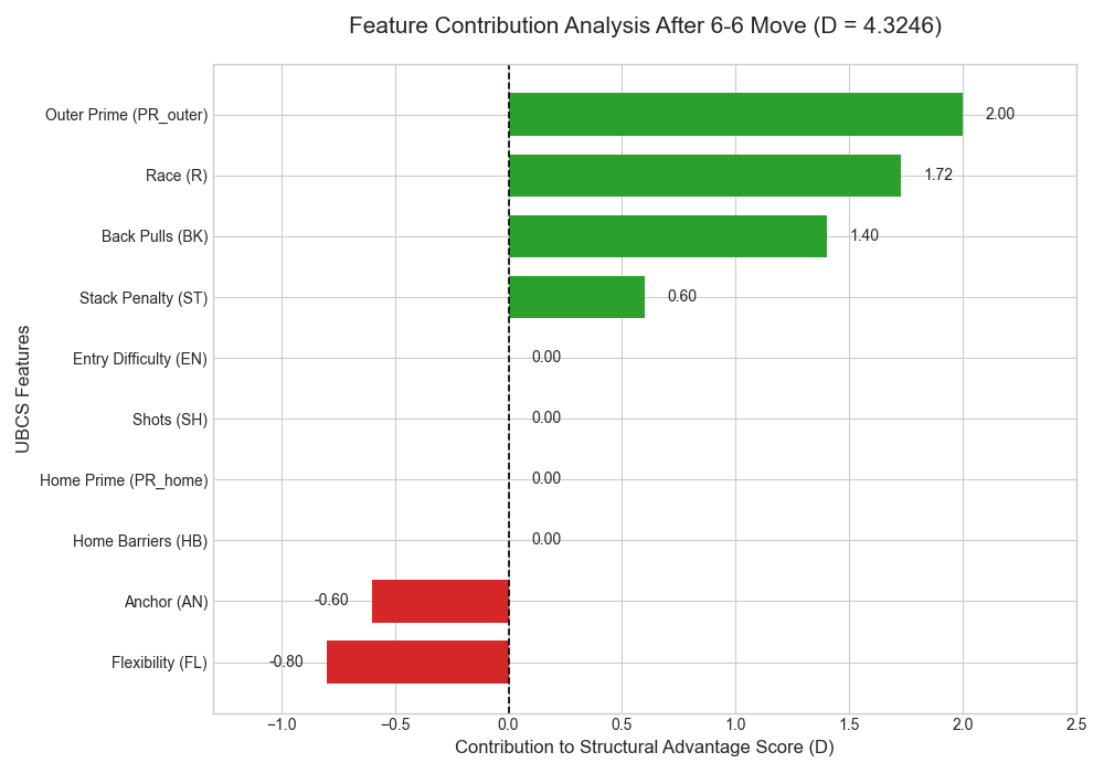
Figure_1.png

Figure_1.png


5. Implementation Blueprint

Pseudocode (single pass, O(24)):

Input: n_you[1..24], n_opp[1..24], b_you, b_opp
Compute P_you = Σ j*n_you[j] + 25*b_you
Compute P_opp = Σ (25-j)*n_opp[j] + 25*b_opp
R = (P_opp - P_you)/167

HB_you = Σ_{k=1..6} h[k] * [n_you[k] ≥ 2]
HB_opp = Σ_{j∈{24..19}} h[25-j] * [n_opp[j] ≥ 2]

PR_home_you  = sum Tri(run_len of closed in {1..6})
PR_outer_you = sum Tri(run_len of closed in {7..12})
PR_home_opp  = sum Tri(run_len of closed in {24..19})
PR_outer_opp = sum Tri(run_len of closed in {18..13})

AN_you = Σ_{j∈{19..24}} a[j] * [n_you[j] ≥ 2]
AN_opp = Σ_{k=1..6} a[25-k] * [n_opp[k] ≥ 2]

SH_you = sum over opp blots j of p(#distinct d in {1..6} with you checker at j+d)
SH_opp = sum over your blots j of p(#distinct d in {1..6} with opp checker at j-d)

c_you = # closed opp points in {24..19}
c_opp = # closed your points in {1..6}
EN_you = b_you * (c_you/6)^2
EN_opp = b_opp * (c_opp/6)^2

FL_you = Σ_{7..13} spare(n_you) + 0.5*Σ_{14..18} spare(n_you)
FL_opp = Σ_{12..18} spare(n_opp) + 0.5*Σ_{7..11} spare(n_opp)

ST_you = Σ max(n_you[j]-4, 0)
ST_opp = Σ max(n_opp[j]-4, 0)

BK_you = 1.0*n_you[24] + 0.7*n_you[23] + 0.4*n_you[22]
BK_opp = 1.0*n_opp[1]  + 0.7*n_opp[2]  + 0.4*n_opp[3]

D = w_r*R + w_hb*(HB_you-HB_opp) + w_prh*(PR_home_you-PR_home_opp) +
    w_pro*(PR_outer_you-PR_outer_opp) + w_an*(AN_you-AN_opp) +
    w_sh*(SH_you - SH_opp) + w_en*(EN_opp - EN_you) +
    w_fl*(FL_you - FL_opp) + w_st*(ST_opp - ST_you) +
    w_bk*(BK_opp - BK_you)

SPE = 50 + 50 * tanh(D / sigma)

6. Tuning & Extensions
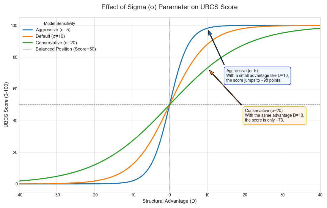
Figure_2.png

Figure_2.png

  • Style bias. Increase (whb,wprh,wan)(w_{hb}, w_{prh}, w_{an})(whb​,wprh​,wan​) for contact‑friendly/human style; increase wrw_rwr​ for racing bias.

  • Variance control. Lower wshw_{sh}wsh​ to de‑emphasize immediate volatility.

  • Learning from data. To map SPE to win% or equity, regress

    atanh⁡ ⁣(SPE−5050)\operatorname{atanh}\!\Big(\frac{\text{SPE}-50}{50}\Big)atanh(50SPE−50​)

    onto engine equities over a training set, learning {w⋅,σ}\{w_\cdot,\sigma\}{w⋅​,σ}.

  • Feature enrichments (future work). Duplication penalties, bear‑off wastage, direct entry combinatorics (beyond (c/6)2(c/6)^2(c/6)2), tempo/roll‑parity terms.


7. Limitations

SPE intentionally uses simple, board‑local features. The shots p(m)p(m)p(m) approximation ignores duplication/legality of specific dice and move‑order constraints; entry difficulty uses a coarse (c/6)2(c/6)^2(c/6)2 proxy; bear‑off wastage and timing are summarized indirectly via race and stacks.


Why Static Positional Evaluation (SPE) and this formula

I’ve wanted to build a transparent, fast, position‑only backgammon score for a long time. Over the past months I surveyed race‑only metrics, rule‑based heuristics, polynomial models, and logistic/softmax scalings. I ultimately chose a two‑part formulation:

  1. Linear structural advantage. D=∑iwi ΔfiD=\sum_i w_i\,\Delta f_iD=∑i​wi​Δfi​ over domain‑grounded, checker‑combination features (race; made points; prime lengths via triangular numbers; anchors; immediate shots; entry difficulty; flexibility; stack penalties; back men). Linear additivity keeps attribution clear, weights tunable, and computations O(24)O(24)O(24).

  2. Bounded, symmetric mapping. SPE=50+50 tanh⁡(D/σ)\text{SPE}=50+50\,\tanh(D/\sigma)SPE=50+50tanh(D/σ). I preferred tanh over logistic, z‑score, or piecewise‑linear scales because it is (a) bounded to an interpretable 0–100, (b) symmetric around 50 (mirrors the opponent’s view), (c) smooth/monotone for stable rankings, and (d) calibration‑friendly via σ\sigmaσ or regression on engine equities.

Conclusion

SPE offers a transparent, fast, and tunable checker‑combination scoring for backgammon with an intuitive 0–100 output. It captures the key structural elements—race, primes, anchors, builders, bar/entry dynamics, stacks, back men—and performs sensibly on standard openings like 6–6.


Related Posts

The Effect of Resonance and Damping on Dynamic System Stability: A Numerical Approach
Jun 7, 2025
Antik Çağlardan Günümüze Yalova'nın Zengin Tarihi
Mar 21, 2025•
yalova-tarihiantik-pylai